Deep Learning Models for IDS with the NSL-KDD dataset
![]()
![]()
![]()
![]()
![]()
![]()
![]()
Abstract
This work is inspired to the paper “Intrusion Detection System for NSL-KDD Dataset Using Convolutional Neural Networks”, DING Yalei and ZHAI Yuqingof, of 2018 2nd International Conference on Computer Science and Artificial Intelligence, which deals with the reproduction of deep learning models on the NSL-KDD dataset. The task is a classification of network attacks, based on network traffic informations. The paper offers a new approach, respect the previous ones, by introducing a CNN-based model with multi-stage features. The goal of this work is to find and compare data processing and ML/DL models, in terms of accuracy rate and true/false positive rate.
Introduction
The project folder is structured in the following way: Data - Folder containing the training and test dataset files img - Folder containing the plots and the schemas images of the work Best_NN - Folder with the callback file of the best NN model weigths Best_CNN - Folder with the callback file of the best CNN model weights NSL-KDD.ipynb - Jupyter notebook of the work Documentation.pdf - This file The dataset analyzed is the NSL-KDD benchmark dataset. As a single attack sends multiple packets, analyzing a single line is not enough, but we need to remember some previous information. For this purpouse is best to use a LSTM (Long Short Term Memory) network based approach. However, two models are tried first, a basic model, Random Forest, and a conventional Feedforward Neural Network model.
Dataset Study
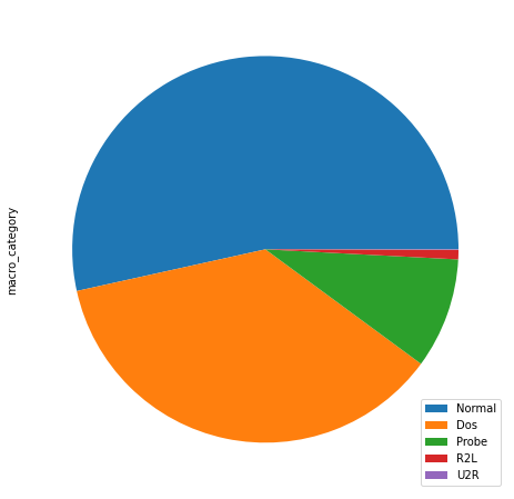
The NSL-KDD benckmark dataset considered in this work is composed by a training file (KDDTrain+.txt) and a test file (KDDTest+.txt). There are 42 attributes: 3 categorical attributes and 39 numerical attributes. Each row describes several features of a network traffic, for example the protocol type and the service used for the connection. The final column of the dataset indicates the category of the traffic. This specific category could identify a type of network attack, or simply a normal traffic. All these categories are grouped into 5 general categories:
- DOS
- PROBE
- R2L
- U2R
- Normal
In the training file, the data distribution in function of categories is very unbalanced. Infact, there are a lot of items with Normal and Dos traffic, but very few cases of U2R and R2L.
Among the main categorical attributes of the dataset, there is the Protocol type: TCP, the transmission control protocol. is used to be sure that the packet is sent to the destination, because a response of the destination reaching is sent back to the sender. UDP, instead, is a protocol used when it’s not necessary to know if the packet reaches the destination. In this way, it is faster than TCP protocol, because there isn’t the response step. ICMP , the Internet Control Message Protocol, is used to check the network state, reachability, and errors. The ping command, for example, uses this protocol and a Dos Attack usually uses the ping command to send a lot of packets to the destination, in order to saturate the resources and to paralize the system. The most frequent protocol used in the training data is TCP, and it is used by all the 5 categories.
The histogram below shows that the ICMP and UDP protocols are used only by Normal traffic, Dos Attacks and Probe Attacks.

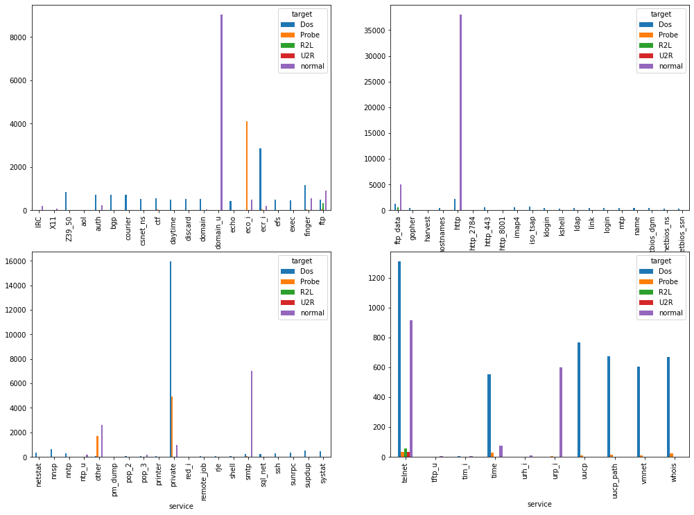
The service feature indicates the kind of service protocol used by the network application. For example, FTP the file transfert protocol used for file transfer, or SMTP used for emails. Each of the five categories uses different services. The most used service protocol is HTTP, which is the web application protocol. Today, this protocol is considered unsure and it is replaced by HTTPS.
The telnet protocol is a network protocol used via command line interface to provide the user with remote login sessions. This protocol is the one used by all five categories, because it is the most vulnerable.
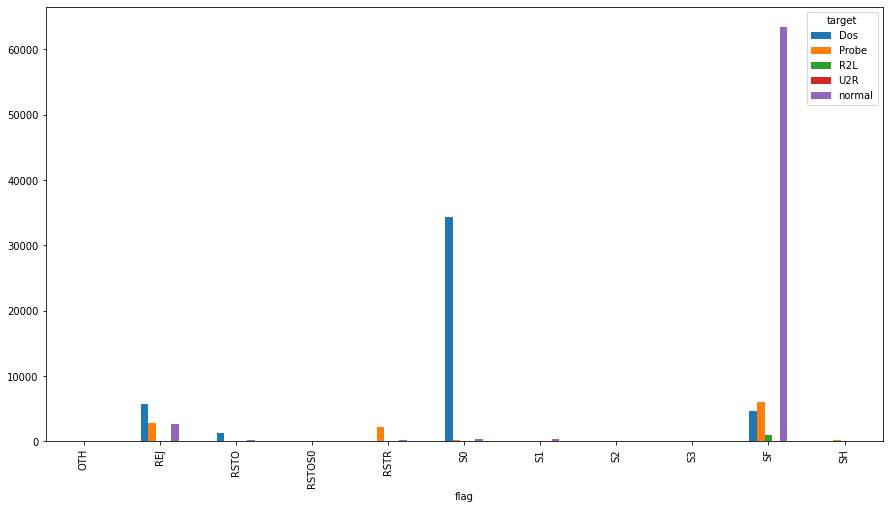
The flag is used to indicate a particular state of connection or to handle a control of a particular connection.
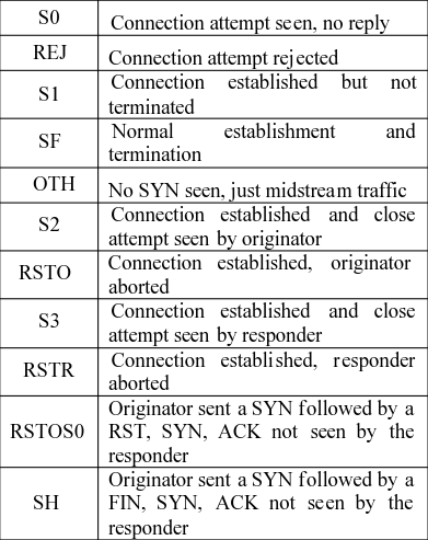
The “S0” flag is widely used by a Dos attack. Infact, the purpouse of Dos attack is to attempt many connection to the server, sending many packets, in order to burden the network load and to make the services unavailables. It doesn’t matter if a connection is established.
Data Preprocessing
ADASYN data augmentation method
In order to have a weighted distribution of label classes, the ADASYN method (Adaptive Synthetic) is used to increase the number of minor frequency classes, according to their difficulty learning level. So, if the original distribution in the training dataset were:
normal 67343
Dos 45927
Probe 11656
R2L 995
U2R 52
after the ADASYN resampling, the final distribution is:
normal 67343
Dos 67238
Probe 67510
R2L 67344
U2R 67336
Data Encoding
The categorical data are encoded into numerical data in the following way: Protocol type and Flag are one-hot encoded. Service is label encoded. So, from an initial number of 42 features, there are now 54.
Data Normalization
Because of the big difference between some columns in terms of scale, a data normalization, the MinMax normalization, is applied on the dataset, in order to keep all the values in the [0-1] range.
$x_{scaled} = \frac{x_i - x_{min}}{x_{max} - x_{min}}$
Models
Evaluation Metrics
The evaluation metrics used in this work are the same as those used in the reference paper.
- Accuracy. the percentage of the records number classified correctly over the total records.
- TPR. True positive rate: percentage of the anomaly records number correctly flagged as anomaly over the total number of anomaly records.
- FPR. False positive rate: percentage of the normal records number wrongly flagged as anomaly is divided by the total number of normal records.
Random Forest Model
The basic model applied to the dataset is Random Forest.
# Model without ADASYN data resampled
RFmodel = RandomForestClassifier(random_state=0)
RFmodel.fit(X_train_scaled, y_train)
RFpredictions = RFmodel.predict(X_test_scaled)
# Model with ADASYN data resampled
RFmodel = RandomForestClassifier(random_state=0)
RFmodel.fit(X_ada_scaled, y_ada)
RFpredictions = RFmodel.predict(X_test_scaled)
The accuracy score of the test prediction is 80,97% with ADASYN resampling, and 76,39% without ADASYN.
The confusion matrix of predicted labels is shown below:

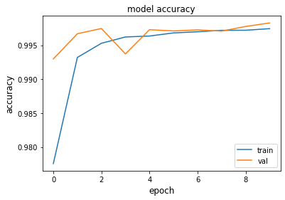
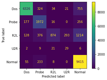
FeedForward Neural Network Model
Three Dense layers of size=256, each followed by Dropout layers with rate=0.2. The best weights of the training are saved to a checkpoint filepath. The final accuracy score, with ADASYN resampled data, is 82.58%, without ADASYN is 79%. The trend of the accuracy/epoch and the confusion matrix are shown below:
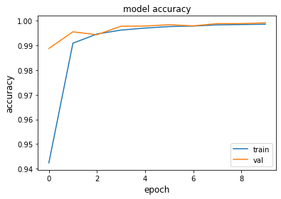
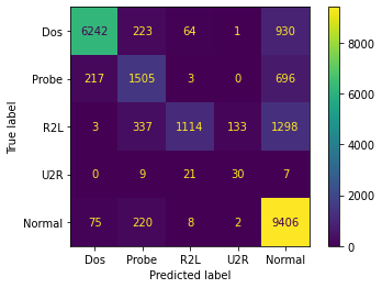
CNN Model
There are three 1D convolutional layers with filters=128 and kernel_size=3, followed by a 1D MaxPooling layer with pool_size=2. Finally a LSTM layer and the Output layer with 5 units and softmax activation function. The best weights of the training are saved to a checkpoint filepath.
The parameters of the training are the following:
- epoch = 10
- batch_size = 64
- Optimization Algorithm = Adam
- Loss = Sparse Categorical Crossentropy
Results
Comparing all the results, in terms of Accuracy, True Positive Rate and False Positive Rate, of this three models plus the paper’s CNN Multistage model (CNN-MSF), we get:
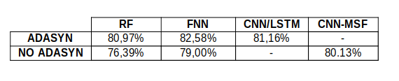
In the first table accuracy values of all models are shown, with ADASYN and NO ADASYN resampling method applied.
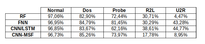
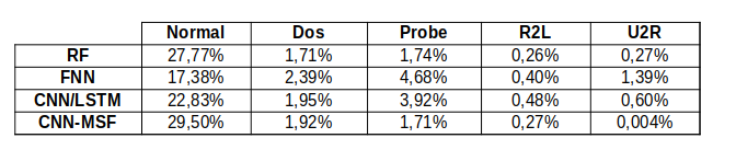
TPR and FPR tables show the values obtained with only ADASYN resampling, because it provided the best accuracy.
An important result is that, with FNN and CNN/LSTM models, the True Positive Rate of U2R predictions goes up over 40%, against the 8,95% of the paper’s model.
Conclusions and future work
The accuracy achieved with ADASYN resampling can be mostly improved by implementing a stacked autoencoder, as described in the paper A Deep Learning Model for Network Intrusion Detection with Imbalanced Data, of 2022. This kind of autoencoders is able to perform dimensionality reduction and enhance data robustness to adapt complex network scenarios.
Ultimately, with the combination of ADASYN resampling, improved stacked autoencoders and LSTM network, 90% accuracy can be achieved.
References
- DING, Yalei; ZHAI, Yuqing. Intrusion detection system for NSL-KDD dataset using convolutional neural networks. In: Proceedings of the 2018 2nd International Conference on Computer Science and Artificial Intelligence. 2018. p. 81-85.
- FU, Yanfang, et al. A Deep Learning Model for Network Intrusion Detection with Imbalanced Data. Electronics, 2022, 11.6: 898.
- NSL-KDD dataset from the Canadian Institute for Cybersecurity.
https://www.unb.ca/cic/datasets/nsl.html
View on GitHub Download as .zip
tags: ids - cybersecurity - deeplearning